Sparklines in Reactable Tables in Shiny Apps
This is the third blog in a series about the {sparkline} R package for inline data visualisations. You can read the first one about getting started with the package here and the second one about embedding them in HTML tables with the {reactable} package here.
In this blog I am taking it a step further and demonstrating how to use our sparkline reactable table in a Shiny app. Thankfully {reactable} has some helpful functions that make this super easy! I will also look at using a dynamic traffic light image in a reactable table at the end.
Reactable Sparkline Table
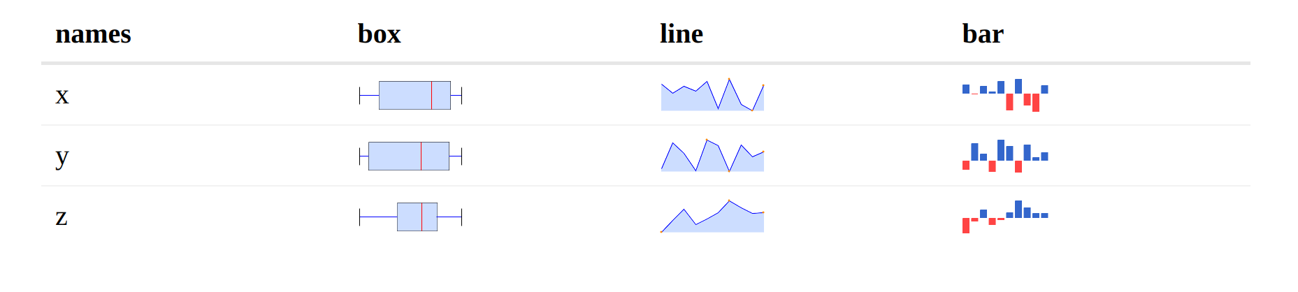
I’m going to start where we ended the last blog. The following code creates a {reactable} table using the iris data with a few {sparkline} visualisations in the columns.
library(sparkline)
library(reactable)
library(dplyr)

data = tibble(
  names = c("x", "y", "z"),
  values = c(list(rnorm(10)), list(rnorm(10)), list(rnorm(10)))
  ) |>
  mutate(box = NA,
         line = NA,
         bar = NA)

table = reactable(data,
          columns = list(
            values = colDef(show = FALSE),
            box = colDef(cell = function(value, index) {
              sparkline(data$values[[index]], type = "box")
            }),
            line = colDef(cell = function(value, index) {
              sparkline(data$values[[index]], type = "line")
            }),
            bar = colDef(cell = function(value, index) {
              sparkline(data$values[[index]], type = "bar")
            })
          )
        )
Using sparklines in a Shiny App
This is actually made very easy by two {reactable} functions which
follow the traditional Shiny naming. In our
server we’ll need to use renderReactable (which uses
htmlwidgets::shinyRenderWidget under the hood), to create our table in
the server. Then in the UI we’ll use reactableOutput (which uses
htmlwidgets::shinyWidgetOutput) to call our table in the app UI.
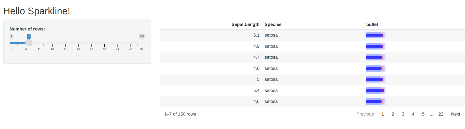
To demonstrate this I am using a basic shiny app with a sparkline bullet chart in a reactable table then a screenshot of the result.
# Server
library(shiny)

server <- function(input, output) {

  output$sparkline_table <- renderReactable({

  data = iris |>
    group_by(.data$Species) |>
    mutate(mean = mean(.data$Sepal.Length),
           lower_range = range(.data$Sepal.Length)[1],
           upper_range = range(.data$Sepal.Length)[2],
           bullet = NA)

  iris_table = reactable(
    d,
    defaultColDef = colDef(show = FALSE),
    columns = list(
      Species = colDef(show = TRUE),
      Sepal.Length = colDef(show = TRUE),
      bullet = colDef(
        cell = function(value, index) {
          sparkline(c(d$mean[[index]],
                      d$Sepal.Length[[index]],
                      d$upper_range[[index]],
                      d$lower_range[[index]]),
                    type = "bullet")
        },
        show = TRUE
      )
    )
  )
  })
}
# UI
ui <- fluidPage(

  titlePanel("Hello Sparkline!"),

  sidebarLayout(
    sidebarPanel = sidebarPanel(
      sliderInput(inputId = "rows",
                  label = "Number of rows:",
                  min = 1,
                  max = 50,
                  value = 30)
    ),

    mainPanel = mainPanel(

      reactableOutput(outputId = "sparkline_table")

  ))
)
Dynamic Image in a Reactable Table
Another thing that you can do with {reactable} is dynamic image columns, to show this I’ve created a traffic light visualisation with 3 levels:
Level 1 (green):

Level 2 (Amber):

Level 3 (Red):

For this example I’m only going to include the code required to create the {reactable} table but following the steps above will work for a shiny app as well, ensuring that the images are available to the app at the path you pass to the table.
The key here is to use a reactable column definition which is a function. This function will take the value and create a html image tag with the path to the correct svg file (png and jpeg will work the same).
library(tibble)
library(htmltools)
library(reactable)

data <- tibble(
    Value = 1:3,
  `Traffic Light` = 1:3
)

path = "/blog/sparkline-reactable-shiny/images/"

table =
  reactable(data,
            defaultColDef = colDef(align = "center"),
            columns = list(`Traffic Light` = colDef(
              cell = function(value) {
                src = paste0(path, value, ".svg")
                image = img(src = src, style = "height: 40px;")
                tagList(
                  div(
                    style = "display: inline-block; width: 60px",
                    image)
                  )
                })
              )
            )
In this blog we have looked at embedding sparkline reactable tables into a shiny app and using another type of dynamic image inside a reactable table. This brings me to the end of the series on {sparkline}, with a notable cameo from {reactable} and a bit of {shiny} too. Stay tuned for similar data science blogs.